The significance of planning for even a small radio network is often neglected. A typical scenario in such cases goes as follows – there’s not enough time (sometimes money) to do proper planning, so the network construction is started right away while decisions on antennas etc. are based mainly on budget restrictions. When the deadline comes, the network is ready but its performance does not meet the expectations. Finally the (expensive) experts are invited to fix the problem and that fix costs ten times more than a proper design process done beforehand would have.
The following paragraphs are not a guide to network planning – that is a topic far beyond the scope of a product manual. What is provided is the essential RipEX data needed plus some comments on common problems which should be addressed during the planning process.
A UHF radio network provides very limited bandwidth for principal reasons. Hence the first and very important step to be taken is estimating/calculating the capacity of the planned network. The goal is to meet the application bandwidth and time-related requirements. Often this step determines the layout of the network, for example when high speed is necessary, only near-LOS (Line-of-sight) radio hops can be used.
RipEX offers an unprecedented range of data rates. The channel width available and signal levels expected/measured on individual hops limit the maximum rate which can be used. The data rate defines the total capacity of one radio channel in one area of coverage, which is shared by all the radio modems within the area. Then several overhead factors, which reduce the total capacity to 25-90% of the “raw” value, have to be considered. They are e.g. RF protocol headers, FEC, channel access procedures and number of store-and-forward repeaters. There is one positive factor left – an optimum compression (e.g. IP optimization) can increase the capacity by 20-200%.
All these factors are heavily influenced by the way the application loads the network. For example, a simple polling-type application results in very long alarm delivery times – an event at a remote is reported only when the respective unit is polled. However the total channel capacity available can be 60-95% of the raw value, since there are no collisions. A report-by-exception type of load yields much better application performance, yet the total channel capacity is reduced to 25-35% because of the protocol overhead needed to avoid and solve collisions.
The basic calculations of network throughput and response times for different RipEX settings can be done at www.racom.eu.
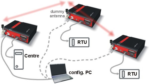
Let us add one comment based on experience. Before committing to the actual network design, it is very wise to do a thorough bench-test with real application equipment and carefully monitor the load generated. A difference against the datasheets, which may be negligible in a LAN environment, may have fundamental consequences for the radio network design. To face that “small” difference when the network is about to be commissioned may be a very expensive experience. The bench test layout should include the application centre, two remotes (at least) and the use of a repeater. See the following picture for an example.
Often the frequency is simply given. If there is a choice, using the optimum frequency range can make a significant difference. Let us make a brief comparison of the most used UHF frequency bands.
160 MHz
The best choice when you have to cover a hilly region and repeaters are not an option. The only frequency of the set of options which can possibly make it to a distant valley, 20 km from your nearest point-of-presence, it can reach a ship 100 km from the shore base. The penalty you pay is tremendous – high level of noise in urban and industry areas, omnipresent multi-path propagation, vulnerability to numerous special propagation effects in troposphere etc. Consequently this frequency band is suitable for low speeds using robust modulation techniques only, and even then a somewhat lower long-term communication reliability has to be acceptable for the application.
350 MHz
Put simply, character of this band is somewhere between 160 and 450 MHz.
450 MHz
The most popular of UHF frequency bands. It still can get you slightly “beyond the horizon”, while the signal stability is good enough for 99% (or better) level of reliability. Multi-path propagation can be a problem, hence high speeds may be limited to near-LOS conditions. Urban and industrial noise does not pose a serious threat (normally), but rather the interference caused by other transmissions is quite frequent source of disturbances.
900 MHz
This band requires planning the network in “microwave” style. Hops longer than about 1 km have to have “almost” clear LOS (Line-of-sight). Of course a 2–5 km link can handle one high building or a bunch of trees in the middle, (which would be a fatal problem for e.g. an 11 GHz microwave). 900 MHz also penetrates buildings quite well, in an industrial environment full of steel and concrete it may be the best choice. The signal gets “everywhere” thanks to many reflections, unfortunately there is bad news attached to this – the reliability of high speed links in such environment is once again limited. Otherwise, if network capacity is your main problem, then 900 MHz allows you to build the fastest and most reliable links. The price you pay (compared to lower frequency bands) is really the price – more repeaters and higher towers increase the initial cost. Long term reliable performance is the reward.
The three frequency bands discussed illustrate the simple basic rules – the higher the frequency, the closer to LOS the signal has to travel. That limits the distance over the Earth’s surface – there is no other fundamental reason why shorter wavelengths could not be used for long distance communication. On the other hand, the higher the frequency, the more reliable the radio link is. The conclusion is then very simple – use the highest frequency band you can.
For every radio hop which may be used in the network, the signal level at the respective receiver input has to be calculated and assessed against requirements. The fundamental requirements are two – the data rate, which is dictated by total throughput and response times required by the application, and the availability, which is again derived from the required reliability of the application. The data rate translates to receiver sensitivity and the availability (e.g. 99,9 % percent of time) results in size of the fade margin.
The basic rule of signal budget says, that the difference between the signal level at the receiver input and the guaranteed receiver sensitivity for the given data rate has to be greater than the fade margin required:
RX signal [dBm] – RX sensitivity [dBm] >= Fade margin [dB]
To calculate the RX signal level, we follow the RF signal path:
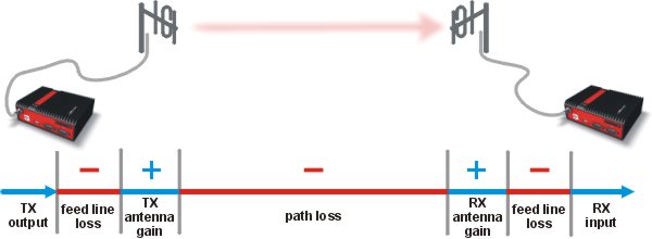
| RX signal [dBm] = | example: | ||
| + TX output [dBm] | +30.0 | dBm (TX output 1 W) | |
| – TX antenna feeder loss [dB] | -2.5 | dB (20m cable RG-213 U, 400 MHz) | |
| +TX antenna gain [dBi] | +2.1 | dBi (half-wave dipole, 0 dBd) | |
| – Path loss [dB] | -125.0 | dB (calculated from field measurement) | |
| + RX antenna gain [dBi] | +9.7 | dBi (7-el Yagi antenna, 7.6 dBd) | |
| – RX antenna feeder loss [dB] | -3.1 | dB (10 m cable RG-58 CU, 400 MHz) | |
| = -88.8 | dBm Received Signal Strength (RSS) | ||
The available TX output power and guaranteed RX sensitivity level for the given data rate have to be declared by the radio manufacturer. RipEX values can be found in Table 5.7, “Maximal power for individual modulations” and in Section 5.4.1, “Detailed Radio parameters”. Antenna gains and directivity diagrams have to be supplied by the antenna manufacturer. Note that antenna gains against isotropic radiator (dBi) are used in the calculation. The figures of feeder cable loss per meter should be also known. Note that coaxial cable parameters may change considerably with time, especially when exposed to an outdoor environment. It is recommended to add a 50-100 % margin for ageing to the calculated feeder loss.
The path loss is the key element in the signal budget. Not only does it form the bulk of the total loss, the time variations of path loss are the reason why a fade margin has to be added. In reality, very often the fade margin is the single technical figure which expresses the trade-off between cost and performance of the network. The decision to incorporate a particular long radio hop in a network, despite that its fade margin indicates 90 % availability at best, is sometimes dictated by the lack of investment in a higher tower or another repeater. Note that RipEX‘s Auto-speed feature allows the use of a lower data rate over specific hops in the network, without the need to reduce the rate and consequently the throughput in the whole network. Lower data rate means lower (= better) value of receiver sensitivity, hence the fade margin of the respective hop improves. See the respective Application note to learn more on the Auto-speed feature. Apart of Auto-speed, there is a possibility from fw ver. 1.6 to set certain Radio protocol parameters individually for a specific radio hop (Individual link options). For more see Section 7.3.2, “Radio”.
When the signal path profile allows for LOS between the TX and RX antennas, the standard formula for free-space signal loss (below) gives reliable results:
Path loss [dB] = 20 * log10 (distance [km]) + 20 * log10 (frequency [MHz]) + 32.5
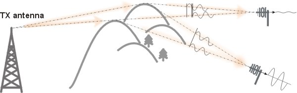
In the real world the path loss is always greater. UHF radio waves can penetrate obstacles (buildings, vegetation), can be reflected from flat objects, can bend over round objects, can disperse behind sharp edges – there are numerous ways how a radio signal can propagate in non-LOS conditions. The additional loss when these propagation modes are involved (mostly combined) is very difficult to calculate. There are sophisticated methods used in RF design software tools which can calculate the path loss and its variations (statistical properties) over a computer model of terrain. Their accuracy is unfortunately very limited. The more obstacles on the path, the less reliable is the result. Such a tool can be very useful in the initial phase of network planning, e.g. to do the first network layout for the estimate of total throughput, however field measurements of every non-LOS radio hop should be done before the final network layout is designed.
Determining the fade margin value is even more difficult. Nevertheless the software tools mentioned can give some guidance, since they can calculate the statistical properties of the signal. Generally the fade margin (for given availability) is proportional to the difference between the real path loss and the LOS path loss over the same distance. Then it is about inversely proportional to frequency (in the UHF range at least). To give an example for 10 km, non-LOS, hop on 450 MHz, fade margin of 20 dB is a bare minimum. A field test may help again, provided it is run for longer period of time (hours-days). RipEX diagnostic tools (ping) report the mean deviation of the RSS, which is a good indication of the signal stability. A multiple of the mean deviation should be added to the fade margin.
Multipath propagation is the arch-enemy of UHF data networks. The signal coming out of the receiving antenna is always a combination of multiple signals. The transmitted signal arrives via different paths, by the various non-LOS ways of propagation. Different paths have different lengths, hence the waveforms are in different phases when hitting the receiving antenna. They may add-up, they may cancel each other out.
What makes things worse is that the path length changes over time. Since half the wavelength – e.g. 0.3 m at 450 MHz – makes all the difference between summation and cancellation, a 0.001% change of a path length (10 cm per 10 km) is often significant. And a small change of air temperature gradient can do that. Well, that is why we have to have a proper fade margin. Now, what makes things really bad is that the path length depends also on frequency. Normally this dependency is negligible within the narrow channel. Unfortunately, because of the phase combinations of multiple waveforms, the resulting signal may get so distorted, that even the sophisticated demodulating techniques cannot read the original data. That is the situation known to RF data network engineers – signal is strong enough and yet “it” does not work.
That is why RipEX reports the, somewhat mystic, figure of DQ (Data Quality) alongside the RSS. The software demodulator uses its own metrics to assess the level of distortion of the incoming signal and produces a single number in one-byte range (0–255), which is proportionate to the “quality” of the signal. Though it is very useful information, it has some limitations. First, it is almost impossible to determine signal quality from a single packet, especially a very short one. That results in quite a jitter of DQ values when watching individual packets. However when DQ keeps jumping up and down it indicates a serious multipath problem. In fact, when DQ stays low all the time, it must be noise or permanent interference behind the problem. The second issue arises from the wide variety of modulation and data rates RipEX supports. Though every attempt has been made to keep the DQ values modulation independent, the differences are inevitable. In other words, experience is necessary to make any conclusions from DQ reading. The less experience you have, the more data you have to collect on the examined link and use other links for comparison.
The DQ value is about proportional to BER (bit error ratio) and about independent of the data rate and modulation used. Hence some rule-of-thumb values can be given. Values below 100 mean the link is unusable. For a value of 125, short packets should get through with some retransmissions, 150–200 means occasional problems will exist (long term testing/evaluation of such link is recommended) and values above 200 should ensure reliable communication.
The first step is the diagnosis. We have to realize we are in trouble and only a field measurement can tell us that. We should forget about software tools and simply assume that a multipath problem may appear on every non-LOS hop in the network.
These are clear indicators of a serious multipath propagation problem:
directional antennas “do not work”, e.g. a dipole placed at the right spot yields a better RSS than a long Yagi, or rotating the directional antenna shows several peaks and troughs of the signal and no clear maximum
RSS changes rapidly (say 10 dB) when antenna is moved by less than a meter in any direction
ping test displays the mean deviation of RSS greater than 6 dB
DQ value keeps “jumping” abnormally from frame to frame
Quite often all the symptoms mentioned can be observed at a site simultaneously. The typical “beginner” mistake would be to chase the spot with the best RSS with an omnidirectional antenna and installing it there. Such a spot may work for several minutes (good luck), sometimes for several weeks (bad luck, since the network may be in full use by then). In fact, installing in such a spot guaranties that trouble will come – the peak is created by two or more signals added up, which means they will cancel out sooner or later.
The right strategy is to find an arrangement where a single signal becomes dominant, possibly the most stable one. “Sweeping” a directional antenna around the place (in different heights and with different polarization) can tell us where the signals come from. If individual signals come from different directions, there is a good chance a long yagi can solve the problem by selecting just one of the bunch. Finding a spot where the unwanted signal is blocked by a local obstacle may help as well (e.g. installing at a side of the building instead of at the roof).
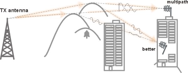
When the multiple signals come from about the same direction, a long yagi alone would not help much. We have to move away from the location, again looking for a place where just one of the signals becomes dominant. 20–50 metres may save the situation, changing the height (if possible) is often the right solution. Sometimes changing the height means going down, not up, e.g. to the base of the building or tower.
We have to remember our hop has two ends, i.e. the solution may be to change antenna or its placement at the opposite end. If everything fails, it is better to use another site as a repeater. Even if such problematic site seems to be usable after all (e.g. it can pass commissioning tests), it will keep generating problems for ever, hence it is very prudent to do something about it as early as possible.
| Note | |
|---|---|
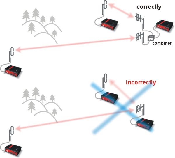
Never design hops where a directional antenna is used for a direction outside its main lobe. However economical and straightforward it may seem, it is a dangerous trap. Enigmatic cases of drop-outs lasting couple of minutes every other day, over a clear LOS hops were created exactly like that. They look like interference which is very difficult to identify and , alas, they are caused by pure multipath propagation, a self-made one. So always use a combiner and another directional antenna if such arrangement is needed. Always. |
In general a radio network layout is mostly (sometimes completely) defined by the application. When the terrain allows for direct radio communication from all sites in the network, the designer can not do too much wrong. Unfortunately for RF network designers, the real world is seldom that simple.
The conditions desirable for every single radio hop were discussed in previous paragraphs. If we are lucky, assuming different layouts meeting those conditions are possible, we should exploit those layouts for the benefit of the network operation. The following options should be considered when defining the layout of a radio network:
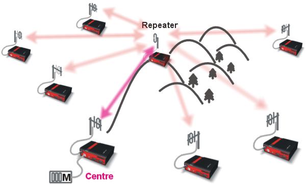
Placing a single repeater, which serves most of the network, on the top of a hill is a straightforward and very common option. Sometimes it is the only feasible option. However, there are a few things we must consider with this design. First, a dominant hilltop site is exposed to interference from a large area; second, these sites are typically crowded with radio equipment of all kinds and it’s a dynamic radio environment, so local interference may appear anytime; third, it makes the majority of communication paths dependent on a single site, so one isolated failure may stop almost the entire network. We need to be careful that these hill top systems are well engineered with appropriate filtering and antenna spacing so that the repeater radios operate under the best possible conditions. Hot Standby repeaters can also improve the repeater integrity. Here is an analogy… It’s hard to have a quiet conversation when a crowd is shouting all around you. So, make sure you give your RipEX repeaters the chance to communicate in a reasonable RF environment. Sometimes a different layout can significantly reduce the vulnerability of a radio network.
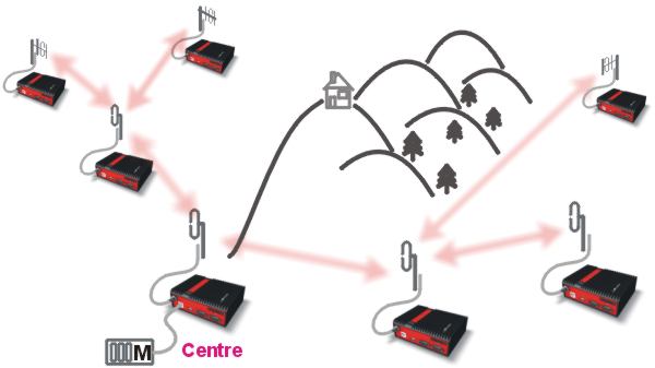
When total throughput is important, as is typical in report-by-exception networks, splitting the network into several independent or only slightly overlapping areas of coverage can help. The placement of repeaters which serve the respective areas is crucial. They should be isolated from each other whenever possible.
in report-by-exception networks the load of hops connecting the centre to major repeaters forms the bottle-neck of total network capacity. Moving these hops to another channel, or, even better, to a wire (fibre, microwave) links can multiply the throughput of the network. It saves not only the load itself, it also significantly reduces the probability of collision. More on that in the following chapter Section 3.6, “Hybrid networks”.
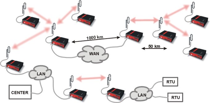
If an extensive area needs to be covered and multiple retranslation would be uneconomical or unsuitable, RipEX units can be interconnected via any IP network (WLAN, Internet, 3G, etc.). This is quite simple because RipEX is a standard IP router with an Ethernet interface. Consequently interconnecting two or more RipEX units over a nested IP network is a standard routing issue and the concrete solution depends on that network.
Let us mention few issues, whose influence on network reliability or performance is sometimes neglected by less experienced planners:
Both vegetation and construction can grow. Especially when planning a high data rate hop which requires a near-LOS terrain profile, take into consideration the possible future growth of obstacles.
When the signal passes a considerable amount of vegetation (e.g. a 100m strip of forest), think of the season. Typically the path loss imposed by vegetation increases when the foliage gets dense or wet (late spring, rainy season). Hence the fade margin should be increased if your field measurements are done in a dry autumn month. The attenuation depends on the distance the signal must penetrate through the forest, and it increases with frequency. According to a CCIR, the attenuation is of the order of 0.05 dB/m at 200 MHz, 0.1 dB/m at 500 MHz, 0.2 dB/m at 1 GHz. At lower frequencies, the attenuation is somewhat lower for horizontal polarization than for vertical, but the difference disappears above about 1 GHz.
Though being a rare problem, moving metallic objects may cause serious disruptions, especially when they are close to one end of the radio hop. They may be cars on a highway, blades of a wind turbine, planes taking off from a nearby airport runway etc.
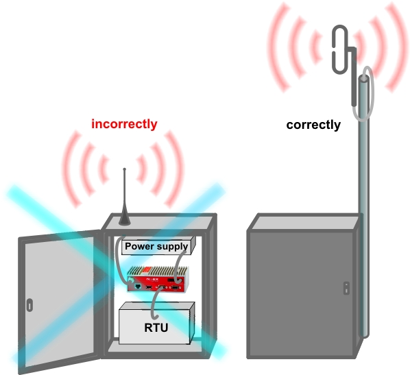
Even when the signal is very strong, be careful when considering various cheap whips or more generally any antennas requiring a ground plane to function properly. A tempting scenario is to use the body of the metallic box, where the radio modem and connected application equipment (often a computer) is installed, as the ground plane, which leads to never-ending problems with locally generated noise. The ground plane forms an integral part of such an antenna, hence it has to be in a safe distance (several metres) from any electronic equipment as well as the antenna itself. A metallic plate used as shielding against interference must not form a part of the antenna.
Do not underestimate ageing of coaxial cables, especially at higher frequencies. Designing a 900 MHz site with 30 m long antenna cable run outdoors would certainly result in trouble two years later.
We recommend to use vertical polarization for all radio modem networks.
To check individual radio link quality run Ping test with these settings: Ping type – RSS, Length [bytes] equal to the longest packets in the networks. Use Operating mode Bridge, when Router, ACK set to Off. Switch off all other traffic on the Radio channel used for testing. The test should run at least hours, preferably day(s). The values below should guarantee a reliable radio link:
Fade margin
Min. 20 dB
Fade margin [dB] = RSS (Received Signal Strength) [dBm] – RX sensitivity [dBm].
Respective RX sensitivity for different data rates can be found in Section 5.4.1, “Detailed Radio parameters”.DQ (Data Quality)
Min. 180PER (Packet Error Rate)
Max. 5 %